Where Matula Tea From

GIS Exercise 4: Spatial Data Processing - Natura 2000

In the fourth GIS exercise, we should use the exercises presented in the previous query and analysis to create a GIS project. The database consists of raster topographic map RLP 100, the vector layers of administrative boundaries of districts of Rhineland-Palatinate and the two vector layers bird sanctuaries (VSG) of Rhineland-Palatinate and the Special Areas of Conservation (Fauna, Flora, Habitat) Rheinland-Pfalz.

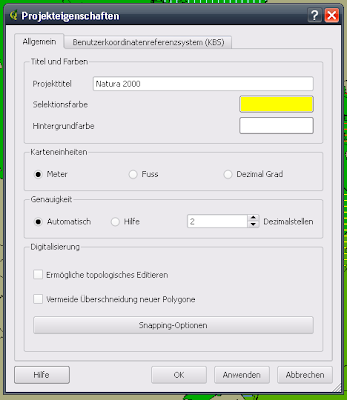
first I met, as always, the project settings. I created a new project, gave the project title ("Natura 2000"), presented the map units to meters and placed the KBS (for Gauss-Kruger zone 2 EPSG 31 466). began

Now I import with which the layer::

general project properties:

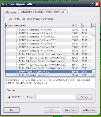
project properties KBS

imported first I the raster layer "TK_100_RLP" and then the three vector layer "kreise_pol.shp", "vsg_rlp_20070111.shp" and "ffh_rlp_20070111. I called this layer next to the default name "LK_RLP" (counties Rheinland-Pfalz), "VSG_RLP (bird sanctuaries Rheinland-Pfalz) and" FFH_RLP (FFH areas Rheinland-Pfalz) around.

Next, several layers are produced with certain requirements.

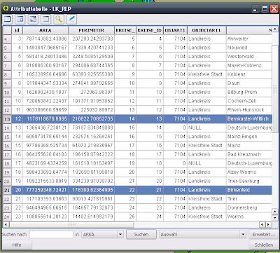
The first was to create a layer that only the two districts Birkenfeld and Bernkastel-Wittlich should contain. For this I first opened the LK_RLP layer attribute table and selected the two districts. In the selection I created a new layer then mithife the button "Save Selection". This layer was named LK_BIR_WIL.shp.

attribute table LK_RLP:

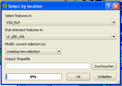
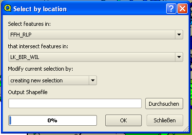
should then create a layer by the bird sanctuaries that are affected by both counties, are shown. For this I chose to Tools / Research Tools / Select by location as the input layer from the Layer VSG_RLP and as an overlay layer LK_BIR_WIL. By clicking OK the new layer was calculated and I was immediately asked if I wanted to import the newly created layer in my project. By confirming the layer was immediately displayed. I renamed this layer in VSG_BIR_WIL.

Creating VSG_BIR_WIL:

The same should now emerge with the FFH-areas that are affected by both counties. For this I chose again from Tools / Research Tools / Select by location. Chose this time as an input layer FFH_RLP, and as an overlay layer LK_BIR_WIL. Also, this layer was calculated by clicking on OK, and after confirmation of whether I want to import this layer also be back in my project displayed. This layer was named FFH_BIR_WIL.

Creating FFH_BIR_WIL:

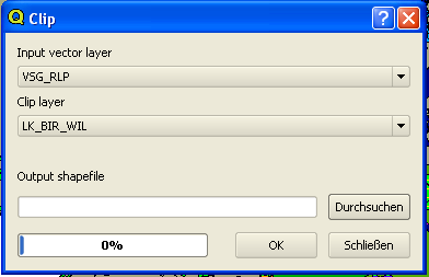
The next step should now only display the bird sanctuaries that are located within the two counties. For this I chose Tools / Geoprocessing Tools / off clip. As an input layer, and I chose the VSG_RLP as clip I selected Layer LK_BIR_WIL. The output shapefile was named VSG_BIR_WIL_clip.shp was calculated after click OK, and then also immediately imported.

Creating VSG_BIR_WIL_clip:

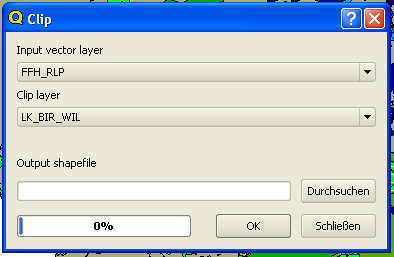
Again, the same should be done with the FFH-areas located within the two districts. For this I again chose Tools / geoprocessing tools from / Clip, chose this time in this menu, but when input layer FFH_RLP and as a clip-Layer LK_BIR_WIL again. This output shapefile was named and was FFH_BIR_WIL_clip.shp and immediately imported into the project.

Creating FFH_BIR_WIL_clip:

Finally, it should be created another layer by the LSG and FFH-areas that are located within the two counties are combined in a new layer. This would normally be possible with the UNION function. The Union function is located in Tools / Geoprocessing Tools / Union

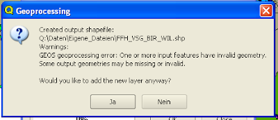
After I set the input layer and the Union in this capacity and had also entered the default name for the new layer and let the program would compute this layer , I got an error message. Therefore, I could not create this layer, unfortunately.

error message in the Union function:

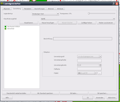
Finally, I cared more about the clarity of the presentation: Right-click on the layer LK_BIR_WIL I chose the menu "Properties". There I clicked on the "View" chose "unique value" as a legend in the classification and type "NAME". Then I clicked yet to "classify" and already I have been in the bar at the left of this menu the districts of Birkenfeld and Bernkastel-Wittlich shown separately. I then chose the two districts each in turn and put in the right area still has a fill color one, so you can distinguish the two districts from one another better.

Layer Properties LK_BIR_WIL:

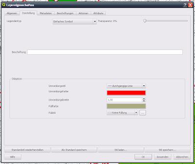
LK_RLP In layer I selected in the layer properties in the representation of any color for the districts, but a border color. The line width of the border, I turned to "1".

Layer Properties LK_RLP:

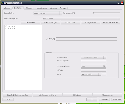
In the Layer VSG_BIR_WIL "I went into the properties menu. There I presented as a legend and type "unique value" and as a classification field "GEBIETSNUM. After clicking on "classification" each site were also displayed. For a full coloration of the bird protection areas would not be particularly useful because the bird protection areas overlap partially with the FFH areas. That is why I chose here a vertical hatching and around the protected areas for birds to be distinguished from each other, I put the hatch on a variety of colors.

Layer Properties VSG:

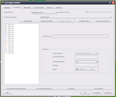
In Layer "FFH_BIR_WIL" I did the same: features menu -> Legend Type "unique value" -> Classification box GEBIETSNUM '-> Classify. Again, I chose a horizontal shading and colored them differently and for different FFH areas.

Layer Properties FFH:

By choosing a vertical hatch for the VSG and a horizontal hatch for FFH-areas can be the areas where an overlap exists makes it particularly easy to identify because there a "diamond pattern" is created.

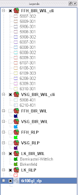
Legend:

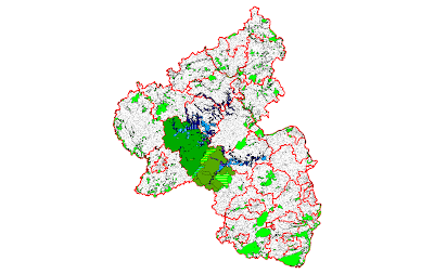
enabled all layers zoomed to Layer LK_RLP:

all the layers selected, click Layer LK_BIR_WIL zoomed:

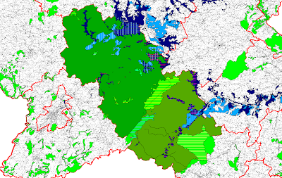
The plan should have the following characteristics:

Topographic Map 100 RLP

county boundaries

LK_BIR_WIL (zoomed to that layer)

VSG_BIR_WIL (by area numbers rated)

FFH_BIR_WIL (classified by region numbers)

Screenshot entire ad:

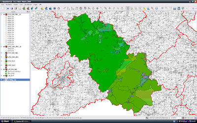
The Score Card:

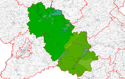
The final plan should now created with the Quick Print feature in PDF format and will be plotted in A2.

The QGIS file, and the whole used and created shape files were burned to a CD and handed in the teaching field.

(Funny, that is not the pictures on my blog can be enlarged. I've uploaded quite normal, but somehow does the enlargement does not. The image of the result card in full resolution, it is well on the CD.)

Hiv Maculopapular Rash Image

GIS Exercise 3: QGIS project building plan TU KL

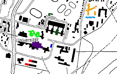
In the third exercise, we should re-create a small project with QGIS. Data base represents a topological map of Kaiserslautern and a shape file "TU_Kaiserslautern" dar.

TU_Kaiserslautern In the file, certain Building (1, 2, 3, 13, 16, 32, 34, 46, 49, 62, 63) of the University are recognized and certain attributes are entered.

After opening QGIS I created first a new project was a project title, the map units set to meters and as a Coordinate Reference System (KBS), I was once again Gauss-Kruger zone 2 (EPSG: 31 466) a.

(This project is the possibility to work either with a vector layer or multiple. First, I will describe how, if we stick to the task within the vector layer TU_Kaiserslautern. Below I will point out the possibility, to work with multiple layers of what you have to paying attention towards this approach and what are the advantages and disadvantages)

project properties. General

Project Properties: Coordinate Reference System (KBS)

After I made these preferences, I added first a layer TK25_6512schw.tif the grid, which should form the data base. Next, I added a layer TU_Kaiserslautern.shp the vector, which we have also been made available.

Next I began trying to capture the individual buildings. For this I chose the vector layer and switch processing status "clicked. Thus, various tools I needed to record the buildings usable. As it was in the area to be covered by buildings, I chose "digitize Polygon from. At first I tried to surround the buildings very well and I zoomed very close to the buildings. For that I needed but a lot of bases and the program crashed several times and my building outline was deleted. After several attempts, I decided to work with fewer points. "Digitize Polygon" The function do you speak about gradually a polyline around the building and the program calculates the resulting surface area developed.

"digitize Polygon

Has my drive around the building completely, simply close the area off with a right click. Then at once the window opens, into which you can enter the attributes of the digitized area just now. We should enter the building number in the "NO" and the relevant department in the "FB". So I went to all buildings prior to and after that, however, were all dyed the same color as I am always in TU_Kaiserslautern layer was. cut out

covered building

order in the buildings 32 and 34, the space in the middle, I turned the layer first in the properties of "representation" is a transparent, so that I areas could see. Then I selected the tool "Add Ring" and covered the land. After a final right-click this previously developed land in my area were cut. Then I turned the transparency off.

Building 49 was not on the topological map of Kaiserslautern, so I drew it free to enter after the submission of building plan.

Next I took care to see the descriptions of each building. They should be labeled with the building number. I dialed in the legend at TU_Kaiserslautern layer by right-clicking the layer properties again, where he went to the "labels" and put the check mark "show labels" to chose the description field "NO" and clicked OK. Thus, even see the building numbers.

Layer Properties: Set the caption

should also we color the building according to the respective departments. For this I chose again from the Layer Properties and clicked the 'Appearance' section. In "Legend Type" I chose the "unique value" and in the classification box I chose "FB" from. Then I clicked on "classification" and each of the individual subject areas was assigned a color. Since I was not particularly happy with these colors, there was one they could not easily distinguished from each other, I chose new colors. This I had to just click on the relevant department in the classification Preview and then change the fill color.

Layer Properties: Set the fill color

Legend:

The QGIS file and the image I burned to CD again to leave everything in the chair.

The finished project:

Screenshot entire screen:

another way: Working with multiple vector layers

Another possibility In this project, working with several vector layers would have been. I would have given the TU_Kaiserslautern.shp file copy multiple times and make a designation of the. Shp files for the respective departments have. The advantage would be that one single vector layer one-off and could and could result see individual departments.

The coloration of the layers in this case would have simply been made using the layer properties to "representation".

The downside would have been that the tax amount increased by the many added. Shp files had. Furthermore, one must in this way the settings for example, the label found in each layer individually.

example of such a legend:

And this work of art in this way:

Replace Mount Targus Tripod

GIS Exercise 2: small QGIS project

In the second exercise, we should create a small QGIS project should have the specific properties and content. Basis represents the topographic map 100 of Rheinland-Pfalz dar. It should be placed several Layer. The administrative boundaries of the districts, unitary councils and local congregations. Finally, a layer should be created with the reserves. The borders of the different administrative boundaries should be consistent with different line width and color are represented. Local communities and protected areas should be marked in appropriate color.

Another benefit should still be zoomed to the local church Weilerbach and a picture of the local community can be created.

The release of QGIS file and the image of Weilerbach was on CD.

After starting QGIS, you must first click on "New Project". The project title should be "Übung_2_ (last name) _ (first name)" for example.

hit The first thing in his new project a few settings: The map units must be in "feet" are provided and the coordinate system must be placed on Gauss-Kruger zone 2. To get into the menu for the preset you have to Settings and then click Project Settings. The map units are then set under "General", the coordinate system under "Coordinate Reference System (KBS) is selected.

project properties:

order now choose to download the map with it, the project is the button "Raster Layer Add "and in the opening menu to select the layer (in this case the card TK100_RLP located in the. tif is format).

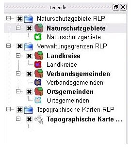
The layer with the administrative boundaries and the nature reserves are on the button" vector layer to add selected "in the QGIS project added. The individual cards I added in succession. For the different cards I created in the legend groups. But you have only a right click in the legend and click on "New Group". I created a group on topographic maps RLP "under I ranks the TK100_RLP. I notified the card in "Topographic Map of 100" to. Next, I created a group for the Administrative boundaries under which I ordered the local communities, municipalities and the Association of Counties. The individual layers to be exactly what I called. As the last group, I created "nature reserves RLP" I class it among the layer with the reserves.

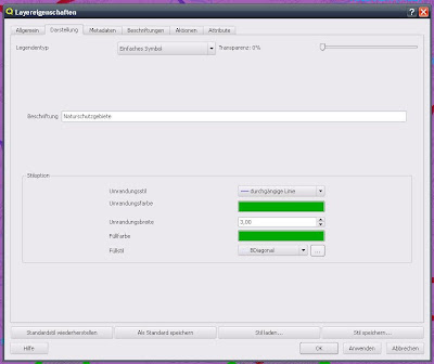
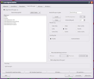
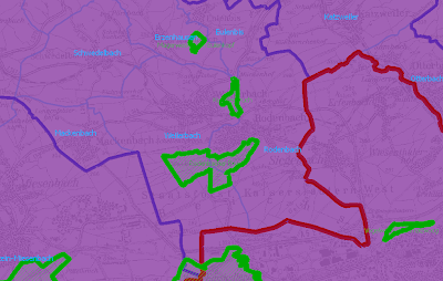
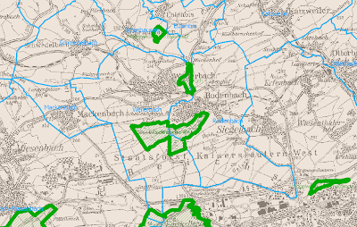
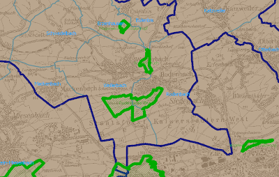
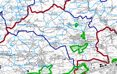
Next I took care of the required layer properties. This I did in the legend for the layer that I wanted to edit just right click and chose "Properties". In the opening menu, I chose the "representation" at the border style, border color and border width set. In the counties and the association communities, I left it at these settings. In local communities and the reserves, I made a few more settings. In local communities, I am still clicked in the box labeled "Check the checkbox to" Show labels on "set. In the Description field, I then had to "NAME" menu. After clicking Apply, have also been shown the names of the local communities. The font size I chose a font size 14 and the font color I chose the same color with which I had outlined in the local communities. With the same approach I made the show the name of the protected area. Only the description field you had here, "GEBIETSNAM" option. In the "View" I selected in the reserves also have a fill color (the same color as the outline and the inscription of the nature reserve) and a fill (BDiagonal). The border width should be different in the three administrative layers. I chose it for the edge width 3 for the counties, border width 2 for the Association of Municipalities and a border width for the local communities, because everything is so beautifully clear, though, switching to the particular zoom level. The protected areas should also be presented with a border width 3.

Layer properties: "display"

Layer Features: "Labels"

Finally, I took care not to change the order of the different layer groups in the legend. The topographical map I placed all the way down, because it is the map. Furthermore, I positioned the administrative borders with a hierarchical order: Local communities - Association of Municipalities - Counties (from bottom to top in the legend). So you can always just click on the desired layer.

Legend:

So you can also view all layers at the same time, I put in the Layer properties of the administrative boundaries still display the transparency. I challenged them each to 40 percent. In the reserves I placed a no transparency because they are in the legend at the top are and thus can be shown always (the color is also so strong). Should I add more layers, I would set the protected areas is also transparent, in this case, this is not absolutely necessary.

As a final point, I zoomed in my practice nor to the local community Weilerbach (to 1:50 000). Selected from all layers and save the image as I in the program to "File" then "Save Image As ..." to clicked. The image was as. png file.

activates all the layers:

- Protected Areas

- Local communities

- Association of Municipalities

- Counties

- Topographic Map 100

The QGIS file and the png. image file from Weilerbach I burned to a CD that I gave then.

more images from Weilerbach On / Off by different layers:

Layer

activated - Local communities

- Protected Areas

- Topographic Map 100

activated Layer:

- Local communities

- Association of Municipalities

- Protected Areas

- Topographic Map 100

result

enabled all layers

Fill the vector layer disabled